
Python专区 加入小组
机器学习还能预测心血管疾病?没错,我用Python写出来了文章代码
使用Python机器学习诊断心血管疾病
1. 商业理解
心血管疾病是全球第一大死亡原因,估计每年夺走1790万人的生命,占全世界死亡人数的31%。
心力衰竭是心血管病引起的常见事件,此数据集包含12个特征,可用于预测心力衰竭的死亡率。
通过采取全人口战略,解决行为风险因素,如吸烟、不健康饮食和肥胖、缺乏身体活动和有害使用酒精,可以预防大多数心血管疾病。
心血管疾病患者或心血管高危人群(由于存在高血压、糖尿病、高脂血症等一个或多个危险因素或已有疾病)需要早期发现和管理,机器学习模型可以提供很大帮助。
2. 数据理解
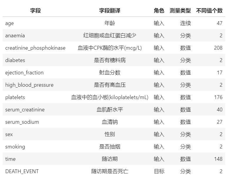
数据取自于kaggle平台分享的心血管疾病数据集,共有13个字段299 条病人诊断记录。具体的字段概要如下:
3. 数据读入和初步处理
首先导入所需包。
# 数据整理
import numpy as np
import pandas as pd

# 可视化
import matplotlib.pyplot as plt
import seaborn as sns
import plotly as py
import plotly.graph_objs as go
import plotly.express as px
import plotly.figure_factory as ff

# 模型建立
from sklearn.linear_model import LogisticRegression
from sklearn.tree import DecisionTreeClassifier
from sklearn.ensemble import GradientBoostingClassifier, RandomForestClassifier
import lightgbm

# 前处理
from sklearn.preprocessing import StandardScaler

# 模型评估
from sklearn.model_selection import train_test_split, GridSearchCV
from sklearn.metrics import plot_confusion_matrix, confusion_matrix, f1_score
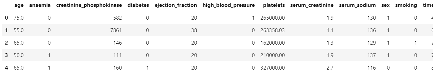
加载并预览数据集:
# 读入数据
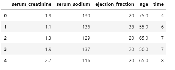
df = pd.read_csv('./data/heart_failure.csv')
df.head()
查看一下数据集概况:
df.info()
<class 'pandas.core.frame.DataFrame'>
RangeIndex: 299 entries, 0 to 298
Data columns (total 13 columns):
age                         299 non-null float64
anaemia                     299 non-null int64
creatinine_phosphokinase    299 non-null int64
diabetes                    299 non-null int64
ejection_fraction           299 non-null int64
high_blood_pressure         299 non-null int64
platelets                   299 non-null float64
serum_creatinine            299 non-null float64
serum_sodium                299 non-null int64
sex                         299 non-null int64
smoking                     299 non-null int64
time                        299 non-null int64
DEATH_EVENT                 299 non-null int64
dtypes: float64(3), int64(10)
memory usage: 30.4 KB
# 查看缺失值
for col in df.columns:
    print(col, ':', str(round(100* df[col].isnull().sum() / len(df), 2)) + '%')
age : 0.0%
anaemia : 0.0%
creatinine_phosphokinase : 0.0%
diabetes : 0.0%
ejection_fraction : 0.0%
high_blood_pressure : 0.0%
platelets : 0.0%
serum_creatinine : 0.0%
serum_sodium : 0.0%
sex : 0.0%
smoking : 0.0%
time : 0.0%
DEATH_EVENT : 0.0%
可以发现,此数据集质量良好,无缺失数据。
4. 探索性分析
4.1 描述性分析
df.describe().T
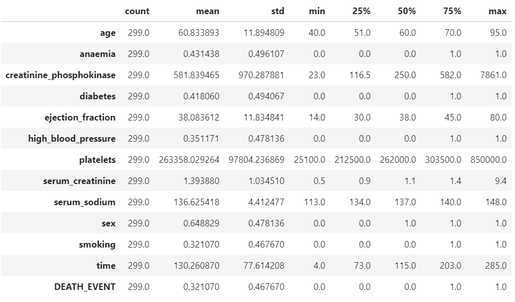
从上述描述性分析结果简单总结如下:
DEATH_EVENT(是否死亡):平均的死亡率为32%;
age:平均年龄60岁,最小40,最大95岁。
diabetes:平均来看,有41.8%患有糖尿病
high_blood_pressure:平均来看,有35.1%患有高血压
smoking:平均来看,有32.1%有抽烟。
4.2 目标变量
# 产生数据
death_num = df['DEATH_EVENT'].value_counts()
death_num = death_num.reset_index()

# 饼图
fig = px.pie(death_num, names='index', values='DEATH_EVENT')
fig.update_layout(title_text='目标变量DEATH_EVENT的分布')
py.offline.plot(fig, filename='./html/目标变量DEATH_EVENT的分布.html')
总共有299人,其中随访期未存活人数96人,占总人数的32.1%
4.3 红细胞、血红蛋白减少和是否存活
bar1 = draw_categorical_graph(df['anaemia'], df['DEATH_EVENT'], title='红细胞、血红蛋白减少和是否存活')
bar1.render('./html/红细胞血红蛋白减少和是否存活.html')
从图中可以看出,红细胞或血红蛋白减少的人群中死亡的概率较高,为35.66%。
4.4 年龄和是否存活
# 产生数据
surv = df[df['DEATH_EVENT'] == 0]['age']
not_surv = df[df['DEATH_EVENT'] == 1]['age']

hist_data = [surv, not_surv]
group_labels = ['Survived', 'Not Survived']

# 直方图
fig = ff.create_distplot(hist_data, group_labels, bin_size=0.5)
fig.update_layout(title_text='年龄和生存状态关系')
py.offline.plot(fig, filename='./html/年龄和生存状态关系.html')
从直方图可以看出,在患心血管疾病的病人中年龄分布差异较大,表现趋势为年龄越大,生存比例越低、死亡的比例越高。
4.5 年龄/性别和是否存活
df.groupby('sex')['DEATH_EVENT'].describe()
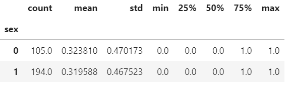
fig = px.violin(df, x='sex', y='age', color='DEATH_EVENT', box=True, points='all', hover_data=df.columns)
fig.update_layout(title_text="年龄和性别与生存状态关系")
py.offline.plot(fig, filename='./html/年龄和性别与生存状态关系.html')
从分组统计和图形可以看出,不同性别之间生存状态没有显著性差异。在死亡的病例中,男性的平均年龄相对较高。
4.6 年龄/是否抽烟和是否存活
df.groupby(['smoking'])['DEATH_EVENT'].describe()
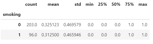
fig = px.violin(df, x='smoking', y='age', color='DEATH_EVENT', box=True, points='all', hover_data=df.columns)
fig.update_layout(title_text="年龄和是否抽烟与生存状态关系")
py.offline.plot(fig, filename='./html/年龄和是否抽烟与生存状态关系.html')
数据显示,整体来看,是否抽烟与生存与否没有显著相关性。但是当我们关注抽烟的人群中,年龄在50岁以下生存概率较高。
4.7 血液中CPK酶的水平与是否存活
fig = px.histogram(df, x='creatinine_phosphokinase', color='DEATH_EVENT', marginal='violin',
             hover_data=df.columns)
fig.update_layout(title_text="血液中CPK酶的水平与生存状态关系")
py.offline.plot(fig, filename='./html/血液中CPK酶的水平与生存状态关系.html')
从直方图可以看出,血液中CPK酶的水平较高的人群死亡的概率较高。
4.8 射血分数和是否存活
fig = px.histogram(df, x="ejection_fraction", color="DEATH_EVENT", marginal="violin", hover_data=df.columns)
fig.update_layout(title_text="射血分数与生存状态关系")
py.offline.plot(fig, filename='./html/射血分数与生存状态关系.html')
射血分数代表了心脏的泵血功能,过高和过低水平下,生存的概率较低。
4.9 血液中的血小板和是否存活
fig = px.histogram(df, x="platelets", color="DEATH_EVENT", marginal="violin", hover_data=df.columns)
fig.update_layout(title_text="血液中的血小板与生存状态关系")
py.offline.plot(fig, filename='./html/血液中的血小板与生存状态关系.html')
血液中血小板(100~300)×10^9个/L,较高或较低的水平则代表不正常,存活的概率较低。
4.10 血肌酐水平和是否存活
fig = px.histogram(df, x="serum_creatinine", color="DEATH_EVENT", marginal="violin",
                   hover_data=df.columns)
fig.update_layout(title_text="血肌酐水平与生存状态关系")
py.offline.plot(fig, filename='./html/血肌酐水平与生存状态关系.html')
血肌酐是检测肾功能的最常用指标,较高的指数代表肾功能不全、肾衰竭,有较高的概率死亡。
4.11 血清钠和是否存活
fig = px.histogram(df, x="serum_sodium", color="DEATH_EVENT", marginal="violin",
                   hover_data=df.columns)
fig.update_layout(title_text="血液中的钠含量和是否存活")
py.offline.plot(fig, filename='./html/血液中的钠含量和是否存活.html')
图形显示,血液中的钠含量较高或较低往往伴随着比较的的风险。
4.12 相关性分析
num_df = df[['age', 'creatinine_phosphokinase', 'ejection_fraction', 'platelets',
                  'serum_creatinine', 'serum_sodium']]

plt.figure(figsize=(12, 12))
sns.heatmap(num_df.corr(), vmin=-1, cmap='coolwarm', linewidths=0.1, annot=True)
plt.title('Pearson correlation coefficient between numeric variables', fontdict={'fontsize': 15})
plt.show()
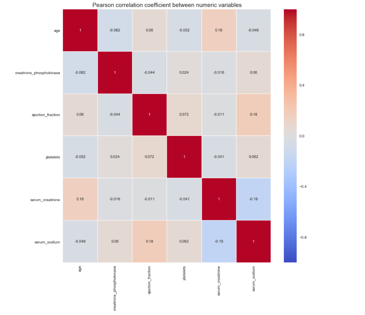
从数值型属性的相关性图可以看出,变量之间没有显著的共线性关系。
5. 特征筛选
我们使用统计方法进行特征筛选,目标变量DEATH_EVENT是分类变量时,当自变量是分类变量,使用卡方鉴定,自变量是数值型变量,使用方差分析。
# 划分X和y
X = df.drop('DEATH_EVENT', axis=1)
y = df['DEATH_EVENT']
from feature_selection import Feature_select

fs = Feature_select(num_method='anova', cate_method='kf')
X_selected = fs.fit_transform(X, y)
X_selected.head()
2020 17:19:49 INFO attr select success!
After select attr: ['serum_creatinine', 'serum_sodium', 'ejection_fraction', 'age', 'time']
6. 数据建模
首先划分训练集和测试集。
# 划分训练集和测试集
Features = X_selected.columns
X = df[Features]
y = df["DEATH_EVENT"]
X_train, X_test, y_train, y_test = train_test_split(X, y, test_size=0.2, stratify=y,
                                                    random_state=2020)
# 标准化
scaler = StandardScaler()
scaler_Xtrain = scaler.fit_transform(X_train)
scaler_Xtest = scaler.fit_transform(X_test)

lr = LogisticRegression()
lr.fit(scaler_Xtrain, y_train)
test_pred = lr.predict(scaler_Xtest)

# F1-score
print("F1_score of LogisticRegression is : ", round(f1_score(y_true=y_test, y_pred=test_pred),2))
F1_score of LogisticRegression is : 0.63
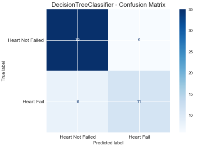
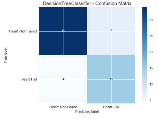
我们使用决策树进行建模,设置特征选择标准为gini,树的深度为5。输出混淆矩阵图:在这个案例中,1类是我们关注的对象。
# DecisionTreeClassifier
clf = DecisionTreeClassifier(criterion='gini', max_depth=5, random_state=1)
clf.fit(X_train, y_train)
test_pred = clf.predict(X_test)

# F1-score
print("F1_score of DecisionTreeClassifier is : ", round(f1_score(y_true=y_test, y_pred=test_pred),2))

# 绘图
plt.figure(figsize=(10, 7))
plot_confusion_matrix(clf, X_test, y_test, cmap='Blues')
plt.title("DecisionTreeClassifier - Confusion Matrix", fontsize=15)
plt.xticks(range(2), ["Heart Not Failed","Heart Fail"], fontsize=12)
plt.yticks(range(2), ["Heart Not Failed","Heart Fail"], fontsize=12)
plt.show()
F1_score of DecisionTreeClassifier is : 0.61
<Figure size 720x504 with 0 Axes>
使用网格搜索进行参数调优,优化标准为f1。
parameters = {'splitter':('best','random'),
              'criterion':("gini","entropy"),
              "max_depth":[*range(1, 20)],
             }

clf = DecisionTreeClassifier(random_state=1)
GS = GridSearchCV(clf, param_grid=parameters, cv=10, scoring='f1', n_jobs=-1)
GS.fit(X_train, y_train)

print(GS.best_params_)
print(GS.best_score_)
{'criterion': 'entropy', 'max_depth': 3, 'splitter': 'best'}
0.7638956305132776
使用最优的模型重新评估测试集效果:
test_pred = GS.best_estimator_.predict(X_test)

# F1-score
print("F1_score of DecisionTreeClassifier is : ", round(f1_score(y_true=y_test, y_pred=test_pred),2))

# 绘图
plt.figure(figsize=(10, 7))
plot_confusion_matrix(GS, X_test, y_test, cmap='Blues')
plt.title("DecisionTreeClassifier - Confusion Matrix", fontsize=15)
plt.xticks(range(2), ["Heart Not Failed","Heart Fail"], fontsize=12)
plt.yticks(range(2), ["Heart Not Failed","Heart Fail"], fontsize=12)
plt.show()
F1_score of DecisionTreeClassifier is : 0.73
<Figure size 720x504 with 0 Axes>
输出属性重要性
imp = pd.Series(GS.best_estimator_.feature_importances_, index=X.columns).sort_values(ascending=False)
imp
time                 0.801905
serum_creatinine     0.113566
serum_sodium         0.045173
age                  0.039356
ejection_fraction    0.000000
dtype: float64
使用随机森林
# RandomForestClassifier
rfc = RandomForestClassifier(n_estimators=1000, random_state=1)

parameters = {'max_depth': np.arange(2, 20, 1) }
GS = GridSearchCV(rfc, param_grid=parameters, cv=10, scoring='f1', n_jobs=-1)
GS.fit(X_train, y_train)

print(GS.best_params_)
print(GS.best_score_)

test_pred = GS.best_estimator_.predict(X_test)

# F1-score
print("F1_score of RandomForestClassifier is : ", round(f1_score(y_true=y_test, y_pred=test_pred),2))
{'max_depth': 3}
0.791157747481277
F1_score of RandomForestClassifier is :  0.53
使用Boosting.
gbl = GradientBoostingClassifier(n_estimators=1000, random_state=1)

parameters = {'max_depth': np.arange(2, 20, 1) }
GS = GridSearchCV(gbl, param_grid=parameters, cv=10, scoring='f1', n_jobs=-1)
GS.fit(X_train, y_train)

print(GS.best_params_)
print(GS.best_score_)

# 测试集
test_pred = GS.best_estimator_.predict(X_test)

# F1-score
print("F1_score of GradientBoostingClassifier is : ", round(f1_score(y_true=y_test, y_pred=test_pred),2))
{'max_depth': 3}
0.7288420428900305
F1_score of GradientBoostingClassifier is :  0.65
使用LGBMClassifier
lgb_clf = lightgbm.LGBMClassifier(boosting_type='gbdt', random_state=1)

parameters = {'max_depth': np.arange(2, 20, 1) }
GS = GridSearchCV(lgb_clf, param_grid=parameters, cv=10, scoring='f1', n_jobs=-1)
GS.fit(X_train, y_train)

print(GS.best_params_)
print(GS.best_score_)

# 测试集
test_pred = GS.best_estimator_.predict(X_test)

# F1-score
print("F1_score of LGBMClassifier is : ", round(f1_score(y_true=y_test, y_pred=test_pred),2))
{'max_depth': 2}
0.780378102289867
F1_score of LGBMClassifier is :  0.74
以下为各模型在测试集上的表现效果对比:
LogisticRegression:0.63
DecisionTree Classifier:0.73
Random Forest Classifier: 0.53
GradientBoosting Classifier: 0.65
LGBM Classifier: 0.74
 心血管预测模型数据+代码.zip
-

运行不出来啊